This is a primer on the philosophically interesting aspects of quantum mechanics. Contents:
I. Weird Experimental Results
II. The Formalism
III. The Copenhagen Interpretation
IV. Bohm's Interpretation
The famous weird experiment is the double-slit experiment; however, it’s easier to explain a simpler case involving electron spin. So, here’s something you can do with electrons:
You pass an electron through an inhomogeneous magnetic field (this is produced by a type of magnet, but don’t worry about the details). The field causes the electron to swerve. It is found that all electrons swerve by the same amount, and half of them swerve up, while the other half swerve down. See a video illustration of this.
We explain this by attributing to the electrons a property, their ‘spin’. Half of them have ‘spin up’ (the ones that swerve up), and the other half have ‘spin down.’
If you rotate the apparatus by 90 degrees, and then pass electrons through again, you find that half of them swerve to the left and half to the right. There’s no correlation between whether an electron swerves up or down and whether it will swerve left or right. Let’s say that the electrons that swerved up in the first experiment had ‘spin up in the y direction,’ the ones that swerved down had ‘spin down in the y direction’, the ones that go right we’ll say have ‘spin up in the x direction’, and the ones that go left we’ll say have ‘spin down in the x direction.’ For short, call those properties “y-spin up”, “y-spin down”, etc. Electrons can also be said to have spin up or down in any other direction. An electron’s spin in a given direction can be determined by passing it through an appropriately oriented magnetic field and then putting a screen in front of it that makes a flash where the electron hits (so you can see which way it swerved). So we can call one of these devices with the magnet a ‘spin measuring device’.
Now, here’s some interesting facts about measurements of spin.
| 1. | If you measure an electron’s spin in a given direction, and then you immediately measure it again, you get the same results both times. E.g., if you determined it to have x-spin up, then the second time you measure its x-spin, you will always find it to have x-spin up again. |
| 2. | x-spin and y-spin measurement results are completely unrelated. I.e., if an electron has been found to have x-spin up, and then you measure its y-spin, it has a 50% chance of having y-spin up and a 50% chance of having y-spin down. There is no way of predicting which will happen. |
| 3. | Measuring the y-spin of an electron completely disrupts its x-spin, and vice versa. That is: If you measure an electron to have x-spin up, then you measure its y-spin (doesn’t matter what the result of this is), and then you measure the x-spin again, it is completely random whether it will have x-spin up or down (50% chance of each). Any possible way of measuring the y-spin of an electron (or x-spin) will destroy all information about its x-spin (or y-spin). |
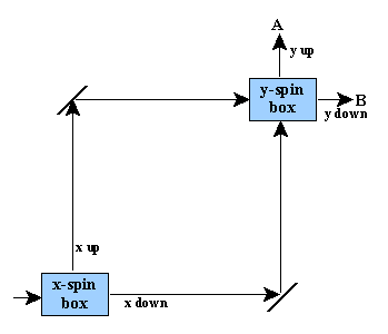
So far, there’s nothing terribly weird. #3 is a bit surprising, perhaps frustrating, but hardly calls for a philosophical revolution, or a revision of classical logic, etc. Now here’s a more exciting experiment you can do. (This is all cribbed from Albert, by the way.) Look at the following setup:
You feed electrons in at the lower left. They go into an x-spin measuring device, which is set up in such a way that the electrons with x-spin up leave the box heading up, and the ones with x-spin down leave the box heading to the right. (This can be verified by feeding electrons with known x-spin up into the device, and putting electron-detectors along the up and right paths.) The electrons going up then bounce off a mirror and get sent to the right, towards the y-spin box. The electrons leaving the x-spin box to the right bounce off a mirror and get sent up towards the same y-spin box.
The y-spin box measures the electrons’ y-spin: y-spin up electrons leave the box going up (path A), and y-spin down electrons leave heading to the right (path B).
Based on points #1-3 above, what should you expect to happen when you run a stream of electrons through the device? How many should come out along path A, and how many along B?
Well, when they go through the x-spin box, they have their x-spin measured. The ones with spin up take the ‘high’ path to the y-spin box. According to points 2 and 3 above, they will then have a 50% chance of coming out along path A, and a 50% chance of coming out along path B. Similarly, the ones that emerge from the x-spin box with x-spin down take the ‘low’ path to the y-spin box; however, they too should have a 50% chance of having y-spin up and a 50% chance of having y-spin down when they get there. So half of them will emerge at A and half will emerge at B. Thus, all in all, 50% of the electrons going into this device should come out at point A, and the other 50% at point B. Note that this should happen regardless of the initial state of the electrons going into the device. E.g., if we feed in electrons with y-spin up at the lower left, or if we feed in electrons with y-spin down, this shouldn’t make any difference to what we see coming out at the end (since their y-spin will be completely disrupted when they enter the x-spin-box).
If you feed electrons with known x-spin into the device, you get the expected result: 50% emerging at A, and 50% emerging at B.
But if you feed electrons with known y-spin into the device (and therefore unknown x-spin), you get something weird: They will emerge from the device with the same y-spin as they had going in; i.e., the x-spin box, in this case, fails to disrupt the value of the y-spin. So if an electron with known y-spin up goes in, it will, with 100% probability, come out at A. Similarly, one with y-spin down will certainly come out at B. This is what actually happens, contrary to our expectation stated two paragraphs ago.
It gets weirder. The setup as described does not allow us to simultaneously determine x-spin and y-spin of an electron; you know the electrons coming out will have y-spin up if they had y-spin up going in, but you don’t know their x-spin, because you can’t tell whether they took the high path or the low path through the device (they wind up at the same place either way). But suppose you try to modify the device so that you can know this also. So you try this:
You feed electrons that are known to have y-spin up into the device. As discussed, you know that in this case, for some reason, the x-spin box fails to disrupt their y-spin. So to find out the y-spin and the x-spin of an electron simultaneously, you just have to contrive some way of figuring out which path (the ‘high’ path or the ‘low’ path) the electron takes through the device. So you put a little wall in the middle of the low path. All the wall does is absorb electrons that hit it. The electrons traveling the high path should be unaffected. So they should emerge with y-spin up, just as they did when the wall wasn’t there. Of course, you’ll only have 50% as many electrons coming out of the device, since half of them will be hitting the wall; but the ones that do come out can be inferred to have x-spin up (since they took the high path through the device) and y-spin up, simultaneously.
What actually happens if you do this, is that now 50% of the electrons going in hit the wall and stop. 50% go through the high path into the y-spin box. Of those, half (or 25% of the total) come out at A and half come out at B. In other words, the y-spin is completely disrupted (randomized). This is odd, to say the least.
What if you put a little electron-detector along one of the paths, instead of a wall? The electron-detector just detects the presence of an electron passing by, and sends it along its way on the same trajectory.
The same thing happens here: the presence of an electron-detector disrupts the y-spin of the electrons, so that half come out at A and half come out at B. If you remove the electron detector, then 100% come out at A, as before. This is despite the fact that the electron detector, by itself, has no effect on electron spins--that is, if you just measure the y-spin of an electron, pass it through the electron-detector, and then measure the y-spin again, it will not have been disturbed. The electron-detector only disturbs the y-spin of an electron in setups like this one, in which knowing where an electron is would enable you to determine its x-spin.
In general, anything that you do that would enable you to figure out the x-spin of an electron going through the device (or to figure out which path it took through the device) will have the effect of disrupting the y-spin. But if you don’t do anything that enables you to figure that out, then the y-spin is unaffected.
That, basically, is where the weirdness of quantum mechanics derives from--ultimately, it is the need to explain observed phenomena like this that drives (or should drive) all the strange things that are said. One other comment: It might seem like the phenomenon described above is paradoxical, even logically impossible (if it doesn’t seem that way to you, you probably didn’t understand it, so reread it); and it definitely seems that some of the theoretical statements people make in QM are such. Indeed, some have proposed that QM shows that we should revise classical logic. But it is certain that the bare phenomena as just described are not contradictory. This is certain not only because they have actually happened, but because the bare data are simply series of distinct observations, and no set of distinct observations, especially observations occurring at different times, can conflict with each other (what I mean by this is that “A observed X at t1” cannot possibly contradict “B observed Y at t2” where t1 and t2 are different times). So any sense of contradictoriness has to come from theorizing, i.e., from our attempts at giving an explanation of what is behind the observations. The observations themselves cannot imply a contradiction, or a revision of classical logic.
In one sense of the term, “quantum mechanics” refers to a certain algorithm physicists have developed for predicting the results of experiments like the ones just described (and many others). The algorithm involves manipulating a bunch of mathematical objects. The algorithm is extremely successful at predicting experimental results, including some results that are very surprising and impossible according to classical physics. There are no known cases in which quantum mechanics fails. It’s reasonable to think the algorithm is completely reliable.
The interesting questions concern the interpretation of quantum mechanics. An interpretation is a theory that explains the physical reality underlying the formalism--i.e., what sorts of things are physically real, and what do the mathematical objects represent; or if you prefer: what is the nature of the physical reality such that this algorithm would work? (That’s vague, but I discuss two examples of interpretations later.)
What about this formalism? First, a distinction: Let’s use “property” to refer to a dimension along which something can vary (or more broadly: something that can take on multiple values). Use “state” to refer to a particular value of a property. So for example, color is a property, and red is a state. Similarly, position is a property; being-right-here (at a particular point in space) is a state corresponding to that property. Now, about the mathematical objects used in quantum mechanics to represent things:
| I. | The state of a system is represented by a vector. (Aside: There are two ways of doing it, one involving matrices, and one involving functions, which turn out to be equivalent; matrices & functions can be viewed as kinds of vectors.) They call this “the state vector” (a.k.a. “the wave function”). You can think of a vector as like an arrow which has a certain length and points in a certain direction (the vector is an abstract, mathematical object, but you can visualize it with an imaginary arrow). |
| In the case of an electron’s spin, the vectors corresponding to the possible spin states would be arrows with a length of 1, pointing in different directions in a two-dimensional, complex space (“complex” because they use complex numbers, rather than real numbers). Note that there is a single vector for an electron’s spin, not separate ones for x-spin and y-spin. This is important. | |
|
There’s a vector that corresponds to having x-spin up, another one for x-spin down, another for y-spin up, and another for y-spin down; each pointing in a different direction in the vector space. I’ll refer to these vectors as “|x up>”, “|x down>”, etc. Then there are infinitely many other vectors (pointing in different directions) that do not correspond to definite values of either x-spin or y-spin. |
| II. | A property of a system is represented by an operator, which is a kind of mathematical object that ‘operates on’ vectors and gives other vectors as outputs. For instance, there would be an operator corresponding to rotating a vector 50 degrees; another one corresponding to, say, reflecting it about the x-axis; etc. There are infinitely many operators. (Don’t try to understand intuitively why a property would be represented by an operator; don’t take “represented” too literally either; let’s just say that for every property there is an operator that is interestingly related to that property.) |
| There’s a special mathematical relationship between the operator that corresponds to a given property, and the vectors that correspond to the particular values (the states) of that property. The relationship is that those vectors are eigenvectors of the operator. Don’t worry about exactly what that means, but just note that most of the vectors will fail to be eigenvectors of a given operator (i.e., will fail to stand in this special relationship to the operator). | |
| In the case of electron spin, then: there’s an operator for x-spin. It has two eigenvectors, which are |x up> and |x down>. There’s another operator for y-spin, and its eigenvectors are |y up> and |y down>. All of the (infinitely many) other vectors in the space are not eigenvectors for either x-spin or y-spin. This means that they do not correspond to particular states of x-spin or y-spin. | |
| III. | There’s an equation that describes how the state vector (or the wave function) evolves over time normally, the Schrödinger Equation. It is deterministic, meaning that given an initial state vector for a physical system, and no outside interference, the equation determines a unique future evolution of that state vector. |
The algorithm for predicting experiment results goes like this:
| a) | Normally (when a system is not being measured), its state evolves according to the Schrödinger Equation. |
| b) | Say you have some property P, which has its own corresponding operator, OP. Suppose that you take a system that happens to be in an eigenstate of OP (so it has a definite value for P). You then measure property P. Then you will, with certainty, find the system to have the state corresponding to that eigenvector. For example: if the state of an electron is |x up>, which is an eigenvector of x-spin, then if you measure the x-spin of the electron, you will, with certainty, find it to have x-spin up. Similarly, if you take an electron whose state vector is |x down> and measure its x-spin, it will be found to have x-spin down. Etc. This is, of course, what you would expect by common sense--things will be measured to have the states they have. |
| c) | If you have a system which is not in an eigenstate of OP, and you do a measurement of P, then the system will jump to an eigenstate of OP, whereupon rule (b) will apply. Which eigenstate it jumps to will be random, with the probabilities being determined by the state vector before the jump (roughly: if the state vector is close to |x up>, then there will be a high probability of its jumping to |x up>, and a low probability of jumping to |x down>). The rule for calculating these probabilities is known as “the Born rule”. This sudden change in the state vector, upon measurement, is known as the “collapse of the wave function,” or the “state vector collapse.” As you might guess, it’s the source of much discussion and puzzlement. |
Rules (a)-(c) predict the experimental results discussed above. For point #2 in the last section: If you measure the x-spin of an electron, then it will jump to an eigenstate of x-spin (if it wasn’t already), either |x up> or |x down>. Let’s say it is |x up>. If you measure its x-spin again, then, according to rule (b) above, you will, with certainty, find it to have x-spin up.
For point #3 in the last section: The Born rule then predicts that, if the state is |x up> and you measure y-spin, it will have a 50% chance of jumping to |y up> (whereupon you observe the electron to have spin up in the y direction), and a 50% chance of jumping to |y down> (whereupon you observe the electron to have spin down in the y direction). Say it jumps to |y down>. The Born rule predicts that, if you now measure the x-spin again, since the state is now |y down>, it will have a 50% chance of jumping back to |x up> and a 50% chance of jumping to |x down>.
What about the weird experiment in the last section, with the setup with the x-spin box and the y-spin box?
You feed in an electron with |y up>. It goes through the x-spin box. However, its x-spin hasn’t actually been measured yet, because it hasn’t been recorded in any macroscopic object that you could observe. (Note: In fact, the concept of a “measurement” is vague and subject to more than one interpretation. This is one of the things that John Bell made a big deal about; Bell didn’t think it was appropriate for the fundamental physical theory to contain a vague term like “measurement.”) So rules (b) and (c) don’t yet apply. After the electron comes out of the y-spin box at the end, you have it hit a screen at either A or B, whereupon you can see a flash where it hit. At that point, its y-spin has been measured. It comes out |y up>, in accordance with rule (b), since its y-spin wasn’t disturbed.
Next, you put a wall in the lower path. This in effect turns the apparatus into an x-spin measuring device, since the fact that an electron gets through now indicates that it had x-spin up; before, without the wall, nothing about x-spin could be determined, since the electron would wind up at the same place regardless of whether it had x-spin up or x-spin down, so x-spin wasn’t measured. So, in accordance with (c), an electron going through will now jump to an eigenstate of x-spin. Then, when it goes through the y-spin box, it will jump to an eigenstate of y-spin, with 50% probability for each of |y up> and |y down>.
There are many different interpretations of quantum mechanics. The Copenhagen Interpretation (hereafter, CI) is the received view, as much as anything is. It is the one you always hear about in the popular science literature. You commonly hear, in pop science literature, statements like the following:
“Quantum mechanics shows that reality is indeterminate; the law of excluded middle is
false.”
“QM shows that observers create reality.”
“QM shows that the world is governed by chance.”
In fact, some of what I said above in (II) actually assumes the CI (e.g., some interpretations say that the wave function does not actually collapse, or jump to an eigenstate, as in rule (c); it just looks like it does). According to the CI:
| i) | Systems evolve according to Schrödinger, deterministically, when they aren’t being measured. |
| ii) | The state vector collapses, as discussed in (c) above, when a system is measured. |
| iii) | Quantum mechanics is complete: i.e., the state vector is a complete representation of the state of a physical system. There are no other variables that need to be added to the theory. (This is what Einstein and Bohr had their big debate about.) |
| iv) | If a system is in an eigenstate of a given property, then it has the corresponding state. |
| v) | If it is not in an eigenstate of a given property, then it does not have any particular value for that property. This follows from (iii). |
Thus, consider the weird experiment again:
The CI says that when you feed a |y up> electron in, this electron has no determinate value for its x-spin. It isn’t just that we don’t know its x-spin; rather, it does not have an x-spin (in accordance with (iii) and (v) above). In fact, an electron cannot possibly have both an x-spin and a y-spin at the same time, since the |x up>, |x down>, |y up>, and |y down> vectors are different vectors in the same space.
The electron does not acquire a definite x-spin, according to the CI, until its x-spin is measured (e.g., if you put the wall in one path, or you insert electron detectors). If its x-spin is not measured, then it stays in its indeterminate x-spin state, which is simultaneously a determinate y-spin state.
Notice that all this explains the experimental results.
Now, you might not find it too paradoxical to have an electron fail to have a definite x-spin. But note that a similar thing applies to position and momentum (hence the infamous “Heisenberg Uncertainty Principle”): in the same way, and for exactly the same sort of reason, that an electron can’t have a definite value of y-spin and a definite value of x-spin at the same time, an electron cannot have a determinate position and a determinate momentum at the same time. There is no vector in the position-momentum space that would represent such a state of affairs. Thus, if QM is complete (as in (iii)), then it is physically impossible to have a (specific) position and momentum at the same time. This is what Einstein objected to, of course; he felt that quantum mechanics was incomplete, and that there were aspects of reality that weren’t represented by the state vector (so-called “hidden variables”)--such as the exact position of a particle.
Another thing that needs to be mentioned is “superpositions”. First, a definition: what is a “linear combination”: Say you have a collection of vectors, v1, v2, .... Suppose you multiply each of them by some number (not necessarily the same number) and then add them together. The result is called a linear combination of v1, v2, .... This result will be another vector. So, for example, suppose that 3(v1) + 6(v2) = v3: then we can say that v3 is a linear combination of v1 and v2.
Now, it turns out that |x up> is a linear combination of |y up> and |y down>; the vector |x up> is equal to the vector [(1/√2)|y up> + (1/√2)|y down>]. (That’s 1 over the square root of 2 times |y up> plus 1 over the square root of 2 times |y down>.) Similarly, |y up> is a linear combination of |x up> and |x down>.
Suppose you have a system whose state vector is a linear combination of the vectors corresponding to states A and B. E.g., if |A> is the state vector for a system in state A, and |B> is the vector for a system in state B, suppose that you have a system whose state vector is a linear combination of |A> and |B>. In that case, we say that the system’s state is “a superposition of A and B.” Note that this defines “superpositions” in terms of how they’re represented mathematically, not what they are physically. Whatever is going on physically when a system is in a superposition, it is something very strange. A system in a superposition of A and B is not in state A. It’s not in state B either. Very important point: It’s not the case that “it is in A or B but we simply don’t know which”--at least, not according to the CI. Here’s why that would be wrong, according to the CI:
Suppose that you put an electron with initial state |y up> into this apparatus again:
This time, let’s say you measure the x-spin of the electron by putting an electron detector on one of the paths. You then destroy the measurement results and forget what they were. So now no one knows what the x-spin of the electron was. In this case, the electron has a determinate but unknown x-spin. That is, according to CI, it jumped to an eigenstate of x-spin when you did the measurement; before it gets to the y-spin box, it is still in an eigenstate of x-spin. Therefore, CI predicts a 50% probability that it will come out at A with y-spin up, and a 50% probability that it will come out at B with y-spin down.
Notice that this is different from the prediction when the electron has an indeterminate x-spin. If you never measured the x-spin of the electron (again, because you don’t do anything to determine whether it is taking the high or the low path), then the electron will not jump to an eigenstate of x-spin, and so it will still have |y up> when it gets to the y-spin box. So it will come out at A, with 100% probability.
Again, to emphasize the point: The theory predicts different observational results (statistically), depending on whether the electron is in an indeterminate state, or in a determinate but unknown state. Therefore, it is impossible, consistently with the theory, to claim that indeterminate states are just determinate states that we don’t have knowledge of. Physical objects will behave differently in observable ways, depending on whether their states are merely unknown, or indeterminate.
The CI view is that objects in superpositions are objects with indeterminate states. E.g., if a particle is in a superposition of many different locations (as all particles are, really), this means it has no specific location.
Lastly, to explain the major problem with the CI. The CI is a logical contradiction (in classical logic). Suppose an object is in a superposition of A and B, where A and B are two states of the same property. In such a case, the CI says that the system is not in A; nor is it in B (point (v) above). However, the system is in either A or B, for: a linear combination of |A> and |B> is an eigenstate of the property, “having-A-or-B” (that’s the property whose values are “yes,” for systems that are either A or B, and “no,” for systems that are neither A nor B). To see this, reflect that if you do a measurement on the system to find out whether it has A, it is uncertain what result you will get (whether yes or no); if you do a measurement to see whether it has B, the result is likewise uncertain. But if you do a measurement to see whether it has either-A-or-B, you will certainly get the answer “yes.” When the system’s state vector is a linear combination of |A> and |B>, it is 100% certain that it will be found to have either A or B.
So the CI implies that this system is (A or B), but is not A and is not B. That’s a contradiction.
To illustrate the point with this apparatus again:
When the experimenter feeds a y-spin up electron into this device, without measuring the electron’s x-spin, then, before the electron reaches the y-spin box, it is in a superposition of having x-spin up and having x-spin down. It is also in a superposition of being on the high path and being on the low path to the y-spin box. It is not definitely on one or the other. But it also isn’t the case that the electron is simply on neither path (e.g., it teleports to the endpoint)--after all, if you block up both paths, then the electron will never get through. The electron is definitely [either x-spin-up-and-on-the-high-path or x-spin-down-and-on-the-low-path], since a test of whether it had that property would yield the answer “yes” 100% of the time. Thus, the electron isn’t on the high path, it isn’t on the low path, but it is on either the high path or the low path.
Here is a further problem with CI: CI implies that systems containing measuring devices behave fundamentally differently from other physical systems. Measuring devices obey different laws from the rest of physical reality. For systems containing no measuring devices always evolve deterministically (point (i) above). But systems containing measuring devices violate normal Schrödinger evolution, having state vector collapses with random outcomes (point (ii)).
Note: if you take a system in a superposition of A and B, and you do a measurement for which state it has, A or B, then according to CI, you will get either the result “A” or the result “B”. However, based purely on Schrödinger evolution, i.e., without the collapse postulate (ii), this wouldn’t be predicted: rather, what we would predict is that the measuring device would go into a superposition of indicating the result “A” and indicating the result “B”. That is: if measuring devices operated according to the same laws as the rest of physical reality, then measurements on systems in indeterminate states should, themselves, have indeterminate outcomes. Similarly, if human beings obeyed the same laws as the rest of physical reality, then the human observer should also go into an indeterminate state: he should go into a superposition of “seeing the instrument indicating ‘A’” and “seeing the instrument indicating ‘B’”.
(For those in the know: the reason for this is simply the linearity of the dynamics. Let |A>S be the vector corresponding to the system being in state A; |B>S the vector representing the system in state B; |ready>M the vector representing the measuring device in its ready state (i.e., ready to make a measurement--the device is turned on, properly oriented, etc.); |“A”>M the vector representing the measuring device indicating that the system is in state A; and |“B”>M the vector representing the measuring device indicating that the system is in state B. Then, if|ready>M |A>S evolves into |“A”>M |A>Sand|ready>M |B>S evolves into |“B”>M |B>S,it follows from the linearity of the dynamics that a linear combination of |ready>M |A>S and |ready>M |B>S should evolve into a linear combination of |“A”>M |A>S and |“B”>M |B>S. Hence, the measuring-device should wind up in a superposition of indicating “A” and indicating “B”.)
The thesis that measuring devices and/or observers obey different laws from the rest of physical reality seems pretty unbelievable, for which reason the CI in general is unbelievable.
You’ve probably heard of the traditional question as to whether light consists of particles or waves. David Bohm proposed a simple answer to this back in the 1950’s (derived from de Broglie’s idea of a “pilot wave”): According to Bohm, there are both particles and waves (this goes not only for light but for elementary particles in general). So suppose you have a single, isolated electron. The particle (the electron) is located at a particular point in space at any given time; it never has an indeterminate position, nor more than one position, nor no position, etc. Unfortunately, we can’t actually find out the exact location of a particle, but this doesn’t mean it doesn’t have one. The wave (the electron’s “wave function”), on the other hand, is spread throughout space, with different amplitudes at different places. The wave function always evolves according to the Schrödinger Equation, deterministically. The particle moves around, with its motion at any given time being determined by the properties of the wave function at the place where the particle is (roughly: if the wave is increasing in amplitude, over time, in a certain direction, then the particle will move in that direction). There’s also a component of the wave function that corresponds to the electron’s spin; spin isn’t a property of the electron itself but of its wave function.
How does this explain the experimental results in this situation:
First, in the original version of the experiment: You put an electron with y-spin up in. What the x-spin box does is split the electron’s pilot wave into two components (two waves), one of which exits the box upward, and one of which exits to the right. The particle will travel along with one of them (which one it travels with will depend on the particle’s exact position within the wave as it was going into the box). The two wave-pieces then travel along their separate paths until they arrive at the y-spin box, whereupon they combine together again, resulting in the same sort of wave function as we had at the beginning (this combination is implied by the mathematics). Thus, if the original wave function was the one corresponding to y-spin up, then the re-constituted wave function in the y-spin box will be the same, and so it will exit the box at point A.
Second, what happens when you put a little wall in the middle of the lower path? What the wall does, essentially, is to block the wave component that was traveling the lower path--it hits the wall and stops. If the electron was traveling along with that wave component, then, the electron is stopped too. If the electron was going with the other wave component, then it will continue on as before. The difference is that this time, when the electron arrives at the y-spin box, the two components of the wave function will not recombine, since one of them was stopped by the wall. Thus, the electron arriving at the y-spin box will not, this time, behave as a y-spin up electron. It will behave, instead, as an x-spin up electron (because the wave that took the upper path through the device had an x-spin up component; the one that took the low path and hit the wall had an x-spin down component; if the two had come back together, they would have added up to a wave function with a y-spin up component, which is a linear combination of x-spin up and x-spin down). Which means that it will have a 50% chance of exiting at point A, and a 50% chance of exiting at point B (again, which of these happens will depend on the electron’s exact position, which we don’t know).
Third, here’s the tricky part: what about the version of the experiment where you insert an electron-detector on one or both paths, which detects the presence of an electron and then sends the electron on its way? Remember that this has the same effect as the wall--it will make an initially y-spin up electron behave as if it has an indeterminate y-spin (i.e., it will have a 50% chance of exiting at A and a 50% chance of exiting at B). Why does this happen?
Before answering that, I first have to explain two ideas:
First idea: the wave function for a system containing multiple particles does not occupy ordinary, 3-dimensional space. Instead, it occupies configuration space. Configuration space is a mathematical space in which the points represent possible states of a system. If you have a single particle, then the configuration space is 3-dimensional, as you would expect, with the dimensions corresponding to the location of the single particle in different directions in physical space (that is: in this case, the configuration space is just a straightforward mathematical representation of physical space). However, if you have a 2-particle system, then the state or “position” of the system is represented as a point in a six dimensional space: one dimension for the x-location of the first particle, one for the x-location of the second particle, one for the y-location of the first particle, etc. Similarly, if you have a 3-particle system, then you have a 9-dimensional configuration space (with 3 dimensions for each particle). The whole system has a wavefunction, which determines the motion of the system through the configuration space (again, the whole system occupies a single point in that space). As an illustration to clarify this idea, suppose you have two of the three particles just sitting there (in physical space), and one of them is moving along the x axis. Then the system as a whole will be moving just along one of the 9 axes in the configuration space. What if a second particle starts moving along the y axis? Then the system will be moving in a diagonal line in the 9 dimensional space. Etc.
Second idea: What is measurement, anyway? A measurement of property A is an operation that establishes a correlation between the value of A that a system possesses, and the location of something observable. For instance, it might be that you have a measuring device with a little pointer on it, and when the system has property A1, the pointer points to “A1”, while if it has A2, the pointer points to “A2”. Or, you might have a measurement device with an LED readout, in which case the value of A is correlated with the positions of certain photons (which are emitted by the display). If the measuring device is any good, it will establish this sort of correlation between its own state and the state of the system it is measuring. This is a conceptual requirement for “measurements”.
Now, what happens when you measure the location of the electron in the above device: any way in which you can do this--that is, any operation that could possibly count as a “measurement of the location of the electron”--would have to establish a correlation between the position of the electron, and the position of something else. And that necessarily means it would constitute a modification of the shape of the wave function in the configuration space--this must be the case, since the wave function is the only thing that determines the positions of anything. The result of this modification will be that the two halves of the wave function, when the electron arrives in the y-spin box, will no longer overlap in the configuration space (this result is predicted by the mathematics). Thus, they will not combine together, and so the electron will behave according to whichever piece of the wave it happens to be in.
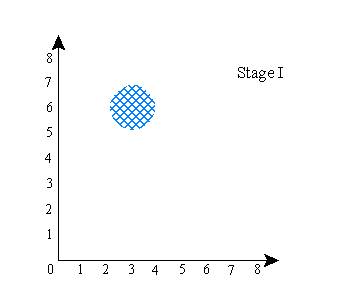
Okay, here will be a simplified explanation of why that happens: First, to make things simpler, let’s pretend that physical space is 1 dimensional, so particles can only move along a single dimension. And let’s suppose you have two particles, call them A and B. The configuration space for this 2-particle system is then a 2-dimensional space. For instance, if the first particle is at x=3 and the second at x=6, then the configuration space looks like this:
The “x” represents the location of the system in the space. Now, let’s suppose that the system’s wave function is what the standard interpretation would call a superposition, specifically, a superposition of [A is at about x=3 and B is at about x=6] and [A is at about x=6 and B is at about x=6]. A’s actual position, let’s say, is x=3. Then the configuration space will look like this:
The shaded region is the region where the wave function has positive amplitude. The “x”, again, is the actual location of the system (the particles) in the configuration space. Notice that in this picture, the positions of A and B are unrelated. That is, if you keep the wave function the same, and imagine particle A in a different place (the system has to be in one of the shaded regions), it has no effect on where particle B is (B would still be at about x=6). Now let’s do a picture in which the locations of A and B are correlated. It would look something like this:
Notice that here, if you keep the wave function the same but put particle A in a different place (i.e., let A be at x=6 instead of x=3), then you also have to move B (particle B would then have to be at about x=2 instead of x=6). So the shape of the wave function (the size and shape of the shaded regions) in this picture guarantees a correlation between the locations of A and B. The shape of the wave function in the previous picture did not.
Now, here’s roughly what happens in the first version of the experiment with the electron, in which you don’t measure the electron’s position: the wave function goes through the following series of stages:
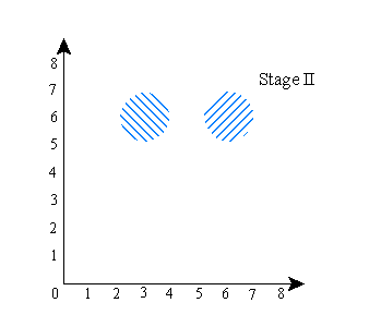
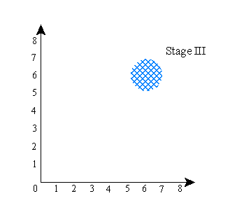
That is: the wave function starts out concentrated in one region (stage I). The device splits the wave into two components (stage II). Finally, the two components are brought back together at a different place (stage III). This is where they recombine to produce the original |y up> state vector. Getting the two parts of the wave to overlap is key. Notice that in all stages, the positions of A and B are unrelated, and in fact nothing at all happens to particle B.
Now, here’s what happens to the wave function if, in the course of the experiment, you do something to establish a correlation between the location of A and the location of B (try to visualize this series taking place in time):
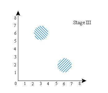
Stage (I) above is the same as the previous stage (I). Stage (II) shows the wave function being split into two components, as before. Stage (III), this time, is the result, after that, of establishing the correlation between the positions of A and B--this is what happens if you use B to “measure” the location of A. Finally (stage IV), the two parts of the wave function are then brought back to x=7 along the horizontal axis, just as they were in the final stage of the previous version of the experiment--only this time, that does not make them overlap in configuration space.
All of this is to explain why taking a measurement (stage III here) makes it so that the two parts of the wave function no longer overlap in configuration space. That explains why, when you take the measurement, you no longer get the weird results (i.e., you will no longer get the electron having |y up> when it gets to the y-spin box). This explanation is simplified, of course, to make it visualizable (chiefly by my omitting several dimensions of configuration space, and ignoring the spin component of the wave function), but this is essentially the reason why the experiment with the y-spin and x-spin boxes comes out the way it does, according to Bohm.
Here are some advantages of Bohm’s theory over the Copenhagen Interpretation:
| 1. | Nothing ever has an indeterminate location, so classical logic need not be abandoned. |
| 2. | Some consider it an advantage that Bohm’s theory preserves determinism. |
| 3. | There is no need to assume that “measurement devices” or “observers” obey different laws from the rest of physical reality. |
Here are some alleged problems with Bohm’s theory:
1. |
It is incompatible with the Special Theory of Relativity in a very clear way (it is not Lorentz invariant). Bohm’s theory implies that there is a preferred reference frame, although there is no experiment we can do to determine which frame it is. However, I have argued previously that quantum mechanics is incompatible with relativity anyway, independent of which interpretation of QM you like (here). |
2. |
The metaphysical status of the wave function in Bohm’s theory is weird. It sounded fine and sensible before I brought in configuration space. But since configuration space probably isn’t physically real (roughly speaking, it’s just a mathematical abstraction), this calls into question whether the wave function is physically real, or what sort of thing the wave function is. This is really a request for clarification of what the theory is. |
3. |
In order to get the right statistical predictions from Bohm’s theory (i.e., the same statistical predictions as standard quantum mechanics), you have to assign a certain sort of probability distribution for the location of a particle (or better, for the location of a system in configuration space)--roughly, that the probability of a particle being located in a region is proportional to the square of the amplitude of the wave function in that region. (More precisely, the probability density = psi-squared.) This posit seems ad hoc and lacks clear motivation. (Note that the probability in question here would be an epistemic probability, relating to our lack of knowledge, or perhaps a frequency-type probability [like that involved in flipping a coin]--not a propensity-type probability [as in the Copenhagen Interpretation].) |
Still, Bohm’s theory shows that it is possible to have a logical explanation of the weird experiments in section (I). At the beginning of (III), I mentioned three major counter-intuitive (not to say crazy) conclusions that are commonly claimed to follow from quantum mechanics, namely:
“Reality is indeterminate; the law of excluded middle is false.”
“Observers create reality.”
“The world is governed by chance.”
Bohm’s theory shows that we don’t have to draw any of these conclusions.
The above exposition is based on a number of miscellaneous sources, including Tim Maudlin’s seminar in the philosophy of quantum mechanics and the following two books. I have relied especially heavily on Albert:
David Z. Albert, Quantum Mechanics and Experience (Cambridge, Mass.: Harvard University Press, 1992).
Tim Maudlin, Quantum Nonlocality and Relativity (Malden, Mass.: Blackwell, 2002).