Solid State NMR

Isotopic Disorder and Many-body Localization

One generally expects waves, both quantum and classical, to propagate well in ordered media and poorly in a disordered environment. The propagation and localization of non-interacting waves in disordered systems has been extensively studied, and is known as Anderson localization in condensed matter physics. We also expect localization of states in disordered many-body interacting systems, but this is a much more complex problem and very little is known about it.

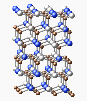
We are trying to explore many-body localization through solid-state nuclear magnetic resonance (NMR) experiments. Our first challenge is to produce coherent quantum systems with well-defined and controllable disorder. The figure at left shows a crystal of silicon carbide. Both carbon and silicon have stable spin-1/2 nuclear isotopes, which can interact with one another through their magnetic dipole moments. They also have stable spin-0 isotopes, and this means we can make a wide range of disordered samples. For example, if we use only carbon-12 (spin-0, shown in brown) and a mixture of silicon-29 (spin-1/2, blue) and silicon-28 or silicon-30 (spin-0, white), we can make a system that is highly ordered with respect to chemical structure but disordered with respect to spin. This is an especially attractive type of disorder because it is fully characterized by isotopic ratios that can be measured accurately. There are many other systems of this type including diamond, silicon, certain minerals such as calcite, and also many organic molecular crystals.

Spin Dynamics

How can we explore many-body localization (and other features of interacting quantum systems) by solid-state NMR? The most common kind of solid-state NMR experiment is aimed at structural analysis. Powder samples and magic-angle spinning are used to average away dipole-dipole interactions so that smaller effects can be observed that more clearly reveal the sample's structure. However, in our experiments quantum evolution under the dipole-dipole interaction is the main interest, so we use single-crystal samples that are not spun.

Consider a collection of $N$ identical spin-1/2 nuclei in a strong magnetic field oriented in the z direction. The two largest terms in the spin Hamiltonian will be the Zeeman interaction with the applied magnetic field and the dipole-dipole interaction between spins. Ignoring smaller effects, the spin Hamiltonian is $$H = -\hbar \omega_0 M^z + H_D,$$ where $M^z=\sum{S_j^z}$ is the total z-component of spin, $\omega_0$ is the Larmor frequency, and $H_D$ is the dipole-dipole interaction. The Zeeman energy per spin is typically 100-500 MHz, while the nearest-neighbor dipole interaction is much smaller, of order 1 kHz.

In thermal equilibrium, the energy eigenstates will be populated according to Boltzmann statistics. The equilibrium quantum state is therefore described by the density operator $$ \DeclareMathOperator{\Tr}{Tr} \rho (0) = {{\exp ({-H \over kT})} \over {\Tr (\exp ({-H \over kT}))}}. $$ NMR is almost always done in the high temperature limit, $kT \gg \hbar \omega_0$. If we expand the exponentials for small arguments and also neglect small effects of $H_D$ on the equilibrium state, the density operator is given by $$ \DeclareMathOperator{\Tr}{Tr} \rho (0) \approx {1 \over 2^N}(\hat{I} + {\hbar \omega_0 \over kT} M^z). $$ For most calculations, the unit operator $\hat{I}$ does not contribute to observables and we are not concerned about overall factors, so it is sufficient to set the initial density operator equal to $M^z$. The Curie factor $\hbar \omega_0 / kT$ tells us that the signal strength will increase at low temperatures and high fields. We use superconducting magnets that generate fields of 7–12 Tesla (proton Larmor freqeuncies of 300–500 MHz). This is within a factor of two of the practical limit. Almost all NMR experiments are done near room-temperature (300 K), but signal strength can be improved by about a factor of 100 by cooling a solid sample to liquid helium temperatures, and experiments at even lower sample temperatures are possible.

We are mainly interested in evolution due to the interactions represented by $H_D$. However, the Zeeman part of the Hamiltonian has three important effects. First, it provides "state preparation", determining the initial density matrix $\rho (0)$ as just described. Second, once the system is disturbed from equilibrium, fast Larmor precession makes the nuclear magnetization observable as an induced voltage in a coil oriented to perpendicular to the applied field. Third, Larmor precession averages away part of any interactions that are present, leaving only "secular terms". This can be seen by transforming to an interaction representation where the Zeeman term vanishes, which is equivalent to adopting a reference frame that rotates around the z-axis at the Larmor frequency. Then operators in $H_D$ that do not commute with $M^z$ will oscillate in time at multiples of the Larmor frequency. It is a good approximation to drop the oscillating terms, leaving the secular dipole-dipole Hamiltonian $$ H_D^s = \sum_{i,j} \hbar \omega_{D}^{i,j}(3 S_i^{z} S_j^{z} - \vec{S}_i \cdot \vec{S}_j), $$ where the sum is over all pairs of spins and $$ \hbar \omega_{D}^{i,j} = -{\mu_0 \gamma^2 \hbar^2 \over 4 \pi r_{i,j}^3}\left({3 \cos^2(\theta_{i,j})-1 \over 2}\right). $$ Here, $\theta_{i,j}$ is the bond angle between spins $i$ and $j$ measured from the z-axis, $r_{i,j}$ is the distance between spins, and $\gamma$ is the gyromagnetic ratio.

With this background, we can describe what happens during a solid-state NMR experiment. As sketched in the figure below, the density matrix is initially equal to $M^z$. The system is then disturbed in some way, for example 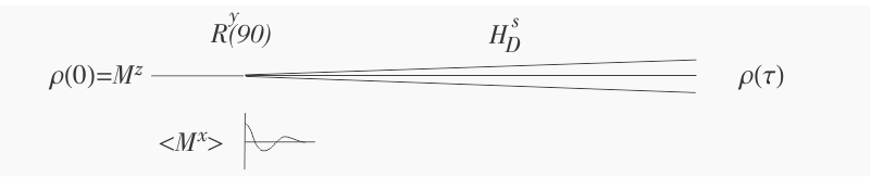by an RF pulse that rotates all of the spins by 90° around the y-axis, so that the density matrix becomes $M^x$ in the rotating frame. (In the lab frame, the transverse magnetization oscillates at the Larmor frequency, and is observable.) The density matrix then evolves under the secular dipolar Hamiltonian $$ \rho (t) = exp(-i H_D^s t) M^x exp(iH_D^s t). $$ After a time $t_{D} \approx \max(\omega_{D}^{-1})$, the terms $M^x=\sum{S_j^x}$ in the density matrix will diminish as nearby spins become correlated, or entangled, and after a time $\tau \gg t_{D}$, many other terms will appear in the density matrix. A general term in $\rho (\tau)$ is a product of Pauli operators $S_i^{x}$, $S_j^{y}$, $S_k^{z}$, and the unit operator $\hat{I}_l$, with one factor for each of the $N$ spins. However, observable magnetization $\left\langle M^x \right\rangle$ is generated only by the un-entangled terms containing a single factor $S_i^{x}$ and $N-1$ unit operators. This is because the expectation value of $M^x$ is $$ \DeclareMathOperator{\Tr}{Tr} \left\langle M^x \right\rangle = \Tr(M^x \rho(t)) $$ and only terms of the form $\DeclareMathOperator{\Tr}{Tr} \Tr(S_i^x S_i^x)$ are non-zero.

The unfortunate consequence of all this is that, just at the time when interesting correlations are beginning to appear in the density matrix, the signal becomes unobservable! A way out of this quandary was discovered by Pines (UC Berkeley) and collaborators in the 1980s. It involves average Hamiltonian theory, Loschmidt echos, and the multi-quantum spectrum.

Average Hamiltonian Theory and the Loschmidt Echo

Suppose we apply a fast pulse to the system that rotates all spins by 90° around the y-axis, and at the same time we rotate our reference frame with the spins so they appear to be unchanged by the pulse. In this "toggling frame", we must transform the spin operators in $H_D^s$ $$ 3 S_i^{z} S_j^{z} - \vec{S}_i \cdot \vec{S}_j \rightarrow 3 S_i^{x} S_j^{x} - \vec{S}_i \cdot \vec{S}_j. $$ If we apply a cyclic sequence of pulses and frame changes like this such that we end up in the original frame, and we do it all quickly compared to $t_{D}$, we can create an average Hamiltonian that differs from $H_D^s$. Methods for doing this, known as average hamiltonian theory, where introduced by John Waugh (MIT) and collaborators in the 1970s. Their famous WAHUHA pulse sequence was designed to average $H_D^s$ to zero, as is often desired in analytical applications of solid-state NMR.

Other sequences can create the Hamiltonian $$ H_{DQ} \propto S_i^{x} S_j^{x} - S_i^{y} S_j^{y} = {1 \over 2}(S_i^+ S_j^+ + S_i^{\raise{1pt}-} S_j^{\raise{1pt}-}). $$ where $S_j^+ = S_j^{x} + i S_j^{y}$ flips the j^th spin up and $S_j^{\raise{1pt} -} = S_j^{x} - i S_j^{y}$ flips it down. This is known as the double-quantum Hamiltonian because it simultaneously flips two coupled spins up or down. Moreover, by a simple change of phase of the pulses is it possible to create $-H_{DQ}$. Evolution under $-H_{DQ}$ is equivalent to time-reversed evolution under $H_{DQ}$, opening the door to creating many-body time-reversal, known in more general contexts as a Loschmidt echo. The experimental scheme is sketched in the figure below.

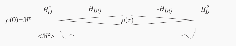
As before, the system starts in the equilibrium state $M^z$. At $t=0$ the double-quantum Hamiltonian is turned on and the magnetization $\left\langle M^z \right\rangle$ quickly decays. At time $\tau$, after extensive correlations have developed in the spin system, the sign of the Hamiltonian is reversed. The system then propagates backwards until an echo of $M^z$ appears at time $2\tau$, when the double-quantum Hamiltonian is switched off. The signal can be observed by converting $M^z$ to $M^x$ with a 90° pulse.

The Loschmidt echo shows that the evolution has indeed been time-reversed and the system has remained coherent for a time $2\tau$. To learn more about the correlated state, we can measure the multi-quantum spectrum. Suppose, at the time $\tau$ when evolution is reversed, we apply a z-rotation to the spin system: $$ \rho(\tau) \rightarrow \exp(-i M^z \phi) \rho(\tau) \exp(+i M^z \phi) $$ To see the effect of this, make a spectral decomposition of $\rho(\tau)$ with respect to $M^z$: $$ \rho = \sum_{m=-N}^{m=+N} \rho_m ; \ \ \ [M^z,\rho_m]=m\rho_m. $$ The quantum number $m$ is called the coherence order. If a term in the density matrix is written as a product of operators $S_i^{z}$, $S_j^+$, and $S_k^{\raise{1pt}-}$, the coherence order of the term is the number of $S^+$ operators minus the number of $S^{\raise{1pt}-}$ operators. Thus a term with coherence order $m$ involves correlations of at least $m$ spins. The rotation labels each component of $\rho(\tau)$ with a phase proportional to its coherence order $$ \rho(\tau) \rightarrow \sum_{m=-N}^{m=+N} \exp(-im\phi) \rho_m(\tau). $$ This phase appears in the echo signal, which is given by $$ \DeclareMathOperator{\Tr}{Tr} \left\langle M^z(2\tau) \right\rangle = \sum_{m=-N}^{m=+N} \exp(-im\phi)\mathcal{I}_m(\tau) ; \ \ \ \mathcal{I}_m(\tau) \equiv \Tr(\rho_{-m}(\tau) \rho_{m}(\tau)), $$ The quantities $\mathcal{I}_m(\tau)$ are called multi-quantum intensities, or collectively the multi-quantum spectrum. They can be determined by repeating the experiment for different $\phi$ and then taking a Fourier-transform with respect to $\phi$.

The multi-quantum spectrum provides a window into the complex entangled state that evolves from an initially uncorrelated equilibrium density matrix. Since the multi-quantum intensity $\mathcal{I}_m(\tau)$ involves at least $m$ spins, it can be used to track how the size of the entangled spin cluster evolves with time, and thus it provides a probe of many-body localization. A pioneering experiment along these lines, using a molecular crystal system with structural disorder, was recently reported by Alvarez, Suter and Kaiser.